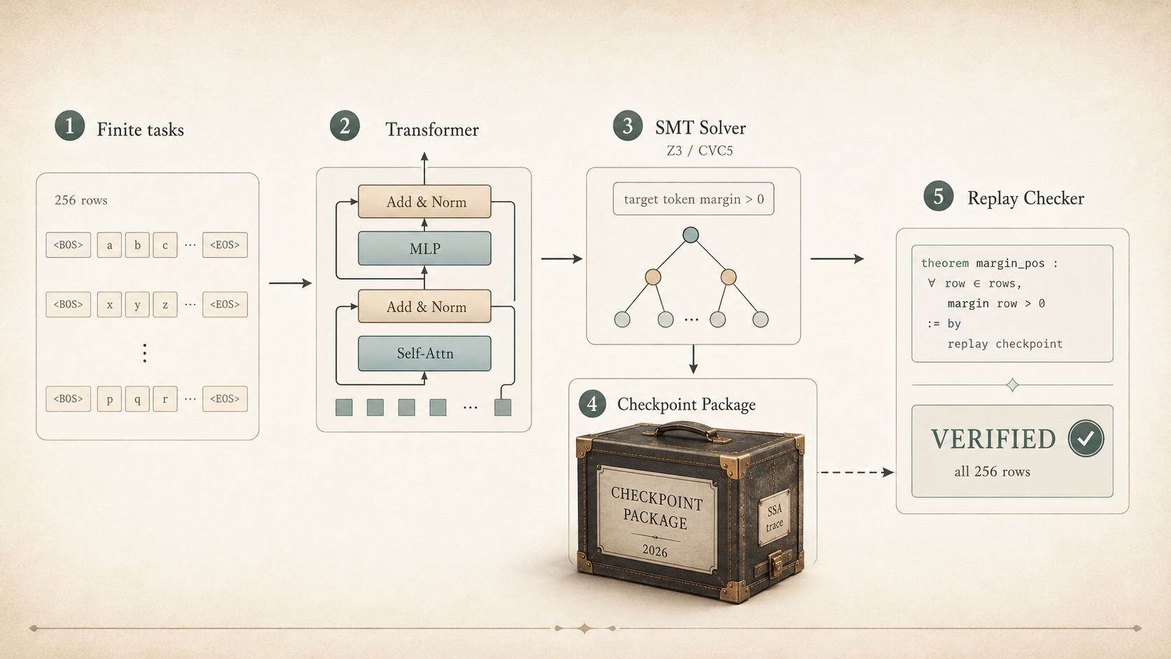
One small GPT style model, a finite symbolic prompt domain, and a Lean/TorchLean layer that checks the exported evidence.
I was reading Neel Somani's verifiable-transformers work (arXiv:2605.24033), and it gave me exactly the kind of test case I wanted for TorchLean. Mechanistic interpretability often points to a circuit and says: this explains the behavior. I wanted to check the next sentence: can the evidence around that claim be made machine-checkable?
Neel's verifier already proves the circuit claims over finite symbolic domains. My question was more practical: after the Python run produces checkpoint files, traces, and summaries, can Lean check that the files I cite still match the claim? If a row is missing, a candidate token is wrong, or a margin turns nonpositive, the build should fail.
Before TorchLean enters the picture, Neel's work is about mechanistic interpretability. A circuit is a small subgraph of a model: a collection of attention heads, MLP features, residual directions, and edges that seems to explain a behavior. A circuit might say "this head copies the opening bracket" or "this MLP feature votes for the quote closing token." Usually that claim is supported by examples, ablations, and human inspection.
The uncomfortable part: an explanation can look right on the cases you checked and fail elsewhere in the domain. For symbolic tasks with finite structure, we should be able to do better, not just "does this circuit seem to work?" but "does this circuit have the claimed property on every input in the declared domain?" Somani's framework converts task localized circuit explanations into bounded propositions a solver can check: formal claims that can be proven or refuted rather than only inspected.
The framework has two verification modes. Direct verification encodes the extracted circuit directly into an SMT solver. When a circuit contains operators that aren't exactly encodable, standard softmax attention for instance, surrogate mediated verification fits a surrogate that SMT can encode, validates it against the original circuit over the bounded domain, and then verifies symbolic explanations against the surrogate. The paper instantiates direct verification on small symbolic sequence tasks using a custom operator stack (BandNorm + sparsemax + LeakyReLU), trains models exhaustively verified on quote closing and bracket type tracking, and demonstrates surrogate mediated verification on circuits extracted from standard attention models. At GPT 2 scale, the same operator stack trains stably on OpenWebText; naive direct SMT verification of full width GPT 2 scale circuits remains intractable. The goal throughout is not full model verification, but a concrete path for turning mechanistic circuit explanations into formal propositions.
Enter the SMT solver
If SMT solvers are not part of your daily life, the basic idea is this: encode the claim as math, then ask the solver to find a counterexample. If it finds one, the claim is false. If it proves no counterexample exists, the claim holds inside the encoded theory.
SMT stands for Satisfiability Modulo Theories. Given a first order formula annotated with a background mathematical theory, the solver decides whether the formula is satisfiable. In other words, is there an assignment to the variables that makes it true? Z3 (from Microsoft Research) is the dominant open source solver. The relevant theory here is Linear Real Arithmetic (LRA): formulas built from linear inequalities over real valued variables, connected by boolean operators like ∧, ∨, ¬.
Z3 handles LRA via DPLL(T), an extension of the classical Davis Putnam Logemann Loveland SAT solving procedure that calls a theory oracle whenever it needs to check consistency of a conjunction of theory literals. For LRA, that oracle is essentially the simplex method. The combination is complete for LRA: satisfiable formulas get a model; unsatisfiable formulas get a proof.
A neural network property like "for all inputs in this set, the correct class has a higher logit than any other" becomes a satisfiability query on the negation: is there an input where some other class wins? The verifier runs Z3 on that negated formula. Either it finds a counterexample (model is sat) or proves there's none (unsat). Linear layers encode into LRA directly as affine constraints. The difficulty is nonlinear activations.
A ReLU introduces one case split per neuron: either the pre activation \(z\ge 0\), with output \(z\), or \(z<0\), with output \(0\). With \(n\) activations, the solver faces up to \(2^n\) branch combinations. Reluplex (Katz et al., 2017) handles this lazily, processing ReLU case splits on demand rather than enumerating all branches upfront. Scaling beyond a few hundred neurons for hard properties remains a challenge.
The piecewise linear boundary: any operator expressible as finitely many affine pieces, including ReLU, LeakyReLU, sparsemax, max pooling, and the BandNorm projection steps, admits an exact LRA encoding via case splits. Exponentials, square roots, and Gaussian CDFs do not. This boundary determines which transformer operators are friendly to SMT.
Verifying a property over a finite input domain shifts the problem structure: instead of proving a universal property over a continuous region, the solver checks each input in the domain (or batches of inputs) as a bounded formula. For a domain of 128 inputs and a circuit with a few dozen activations, the problem becomes tractable.
Why standard Transformers hate solvers
Standard Transformers are rough on SMT solvers for a simple reason: softmax. Softmax uses exponentials, and exponentials are outside Linear Real Arithmetic. Z3 has no complete decision procedure for formulas involving \(e^x\), so encoding softmax exactly is not possible without either adding an uninterpreted function with axioms or using polynomial approximations.
The data dependent square root couples all coordinates through a nonlinear denominator.
GELU has the same flavor of problem: \(\operatorname{GELU}(x)=x\Phi(x)\), where \(\Phi\) is the Gaussian CDF. Even approximate piecewise linear encodings of these operators introduce error that compounds across layers.
Beyond the per operator difficulty, attention's bilinear score computation \(q^\top k\) is quadratic in the inputs. With softmax normalization on top, the solver faces a tangle of mutually dependent nonlinear constraints with few simplification opportunities. Each softmax in each layer adds more transcendental structure; across multiple layers the encoding becomes prohibitively expensive even before accounting for the case split blowup from any approximate piecewise linear treatment.
The architecture choices in verifiable-transformers are a response to exactly this: replace each operator that is hostile to solvers with a piecewise linear or affine equivalent that stays inside the LRA plus case split fragment, without abandoning the transformer skeleton.
The model changes
The model is a GPT style decoder only transformer with pre norm residual blocks and an untied lm_head. Three components differ from standard GPT 2.
Signed L1 BandNorm
BandNorm replaces LayerNorm. Given an input vector x, the algorithm proceeds in six steps:
Center: \(c=x-\operatorname{mean}(x)\)
Sign split: \(p=\max(c,0)\), \(n=\max(-c,0)\), so \(c=p-n\) with \(p,n\ge 0\)
L1 band projection (applied to each of p and n separately): if the L1 mass exceeds an upper band threshold, project onto an L1 ball via coordinate wise thresholding. If mass falls below a lower band threshold after projection, add a bounded lift over the active (nonzero) coordinates.
Recombine: \(z=p'-n'\)
Recenter: \(z=z-\operatorname{mean}(z)\)
Affine: \(\operatorname{out}=\gamma\odot z+\beta\), with learned scale \(\gamma\) and bias \(\beta\)
Every step is a linear operation, a coordinate wise max with 0, or a scalar comparison and threshold. No square roots, no data dependent denominators. The L1 projection in step 3 is piecewise linear: each coordinate is either clipped at a threshold (one case split) or passed through unchanged. The entire normalization operator encodes into LRA plus one case split per coordinate per layer. It is expensive for large widths, but exact.
Sparsemax attention
Sparsemax replaces softmax as the attention normalization. It is the Euclidean projection of the score vector \(s\) onto the probability simplex \(\Delta^{K-1}\).
The threshold \(\tau(s)\) is determined by sorting: choose the largest \(k\) such that \(1+k\,s_{(k)} > \sum_{j\le k}s_{(j)}\), where \(s_{(1)}\ge s_{(2)}\ge\cdots\) is the sorted sequence.
Unlike softmax, sparsemax produces exact zeros, giving sparse attention distributions. More importantly, within each possible active set \(\{i:p_i>0\}\), the operation is affine. The active set itself is determined by a sort and a threshold comparison, so the overall function is piecewise linear. The bilinear score computation \(q^\top k\) remains quadratic in the query and key vectors, which is representable in LRA but grows expensive at larger widths. The paper's tractability results are therefore for the small model setting; at GPT 2 scale the SMT encoding for each circuit becomes intractable.
One case split per neuron. The SMT encoding is a single disjunction between two linear constraints, the simplest possible activation from a verification standpoint.
Each transformer block uses pre norm BandNorm, single head causal sparsemax attention, and a two layer LeakyReLU MLP. The final residual goes through BandNorm and the unembedding matrix.
The four verified properties
For each task, the paper defines a finite exhaustive task domain \(D_{\mathrm{task}}\) and a candidate token set \(T\). For quote closing, the candidates are ' and ". For bracket type, the candidates are ] and }. The task decision \(d_T(F,x)=\operatorname*{arg\,max}_{t\in T}F_t(x)\) is the model's choice among the relevant candidates only, not across the full vocabulary.
The notation is compact but useful: \(P\) is the symbolic reference program, basically a lookup on the opening delimiter. \(C_E\) is the extracted circuit using retained edge set \(E\). \(C_{E\setminus\{e\}}\) is the same circuit after removing one edge. \(r_E(x)\) is the final residual before the output head. \(G_T(r)\) applies BandNorm and the unembedding, then takes the task decision over \(T\).
The colors below separate the four claims: green is agreement with the reference program, orange is edge necessity, blue is content invariance, and violet is numerical robustness.
01 · Agreement
Functional equivalence
\[
\forall x \in D_{\mathrm{task}},\quad
d_T(C_E,x)=P(x)
\]
The circuit's task decision agrees with the reference program on every input in the domain. If this fails, Z3 gives a concrete counterexample.
Every retained edge is behaviorally necessary: removing it changes the task decision on at least one input. This does not prove ACDC found a globally minimal circuit, but it does prove no retained edge is redundant under this test.
The circuit ignores input variation that does not matter for the task. For quote closing, \(R(x,x')\) holds when both prompts share the same opening quote token, so filler tokens cannot flip the decision.
The task decision is stable under bounded \(\ell_\infty\) perturbations to the final residual. The verifier first checks that the traced BandNorm branch remains stable inside the \(\varepsilon\) ball, then checks that the decision cannot flip inside that branch.
Results on the small model: quote closing uses 3 retained edges, bracket type uses 6. Both cover 128 inputs (full exhaustive task domain). All four properties: VERIFIED for both tasks.
Circuit extraction uses ACDC (Automated Circuit DisCovery, Conmy et al. 2023), which iteratively ablates edges from the full computational graph and retains those whose removal changes model behavior above a threshold. The sanity check before SMT verification runs an exhaustive PyTorch forward pass over the task domain using only the retained edges, confirming the extracted circuit still solves the task before any Z3 calls.
The two finite tasks
The model has a 32 token vocabulary, sequence length 6, width 16, 2 layers, 1 attention head, and MLP width 64, roughly 8,000 parameters. At that scale, the entire task domain is enumerable and tractable for SMT.
Two tasks:
quote_close: pick the matching quote token, 9 (single quote ') or 10 (double quote ").
bracket_type: pick the matching closing bracket, 13 (]) or 14 (}).
The finite certificate has 256 prompt rows: 128 quote rows and 128 bracket rows. Each row records the prompt, task label, target token, alternate token, and the margin between the target and alternate logits. The property checked is projected: the target must beat the specific alternate candidate that matters for the task, not the full vocabulary. The projection is appropriate because quote closing only needs to distinguish ' from ", and a claim scoped to that distinction is more precise than a claim about the full output distribution.
This is not a full vocabulary claim. It checks the candidate decision that the symbolic task cares about.
Part
Value
Prompt rows total
256 canonical rows
Quote rows
128, candidates 9 vs 10
Bracket rows
128, candidates 13 vs 14
Decision property
\(z_{\mathrm{target}}>z_{\mathrm{alternate}}\)
Minimum replayed margin
0.019695
The claim is explicitly scoped: on these 256 canonical prompts, for these two candidate token decisions, this checkpoint has positive target over alternate margins when replayed in Lean. Not "the model understands brackets." Something smaller, more checkable, and more useful.
What one row means
This is where the exported trace becomes precise. A row is not “the model got an example right.” A row records one exact prompt: the tokens, the task, the token that should win, the alternate token, and the measured gap between them.
Lean turns that receipt into something stricter. The row has to belong to the finite prompt list we promised to cover. A quote row has to use quote candidates. A bracket row has to use bracket candidates. The target score has to beat the alternate score. Later, the replay recomputes the same decision from the embedded checkpoint values instead of trusting the Python log.
This separates two things that are easy to blur. The Python row is an empirical record. The Lean row is a typed claim with predicates attached. Sampling says “I looked at some examples.” Exhaustive checking says “this declared domain was covered.” For a circuit explanation on a finite symbolic task, those are different standards of evidence.
Why 256 rows matters
It is tempting to dismiss a tiny finite domain as a toy. I do not think that is quite right. Circuit explanations usually start with narrow behaviors anyway: close the matching quote, track bracket type, copy a variable, remember whether a delimiter appeared. Those are not whole language claims. They are local claims about a mechanism in a bounded setting.
So the first serious question is not “does this already scale to every model?” It is “on the domain you claimed, does the mechanism actually explain the behavior?” Here the declared domain has 256 prompts. That is small enough to enumerate, and enumeration is exactly what makes the claim crisp.
This does not prove the model generalizes to arbitrary strings. It does prove that the exported finite trace has the promised shape, row count, task split, checkpoint hash, and positive projected decisions. That is a small claim, but it is a claim you can actually make a machine check.
Making the circuit claim portable
The solver result is not the only thing that can go wrong. The circuit summary has to travel through files, scripts, generated Lean constants, and human-written claims. That is where boring mistakes creep in: a stale checkpoint, the wrong candidate tokens, a copied summary from a previous run, or a trace with one row missing.
Lean is not running Z3 again here. It is doing a different job. Z3 searches the constraint space. Lean checks that the exported evidence is internally consistent: metadata, finite rows, circuit summaries, and the replayed checkpoint all have to agree.
This layer does not replace the solver. It turns “the solver verified something” into a more specific claim: this trace, this checkpoint identity, these circuit summaries, and these replayed decisions all line up.
Why I added Lean
Z3 and Lean are not competing here. Z3 handles the mathematical search: is there a counterexample to the circuit claim on the bounded domain? Lean handles the evidence boundary: did the files we are publishing actually come from the same run, with the same checkpoint, the same row order, the same candidate convention, and the same positive margins?
This boundary matters because experiments have plumbing. A notebook can print PASS while a stale generated file points to yesterday's checkpoint. A trace can look plausible while missing a row. A summary can report zero failures while using the wrong task candidates. Lean is useful here because the final statement goes through only if the generated constants and predicates line up.
What Lean checks
The Lean layer turns the exported run into data that the kernel can check. The check has five layers, each catching a different kind of mismatch:
Identity
Model name, architecture, operator choices, tensor names and shapes, parameter count, checkpoint fingerprint.
Coverage
256 canonical prompt rows with the expected quote/bracket split.
Margins
Target token, alternate token, positive target over alternate margin per row.
Circuits
Quote and bracket summaries: retained edge count, verified case count, robustness radius, zero failures.
Replay
Neel's exported checkpoint values replayed in Lean Float over all 256 finite prompts.
TorchLean
Same shape TorchLean native run emitting a trace checked by the same finite decision contract.
The generated Lean files still exist, of course, but the more interesting part is the discipline they force. Rename a tensor, change a shape, drop a prompt row, swap a candidate token, or let a margin go nonpositive, and the final checked statements stop compiling. The files are accepted only insofar as the predicates accept them.
The boring bugs that matter
Let's be honest: the bugs that ruin experiment writeups are often not profound mathematical paradoxes. They are stupid things. A checkpoint changes but the generated summary still names the old fingerprint. A script emits 255 rows instead of 256. The quote task accidentally uses bracket candidate tokens. Target and alternate are swapped. The TorchLean trace comes from the wrong saved parameter file.
None of these require deep mathematics to detect. They require discipline. I added the Lean layer because I wanted the build to stop me from citing outdated files as if they were current.
Mistake
Why it matters
Where it fails
wrong checkpoint identity
evidence may refer to a different model
export summary check
missing prompt rows
finite domain coverage claim is false
evaluation trace check
wrong candidate tokens
projected decision checks wrong property
row/task predicate
nonpositive margin
target doesn't beat the alternate
margin predicate or replay
stale circuit summary
solver side result may not match exported run
verification summary check
Replaying the checkpoint
The strongest check is the forward replay. Replay/UpstreamFloatReplay.lean embeds Neel's checkpoint values as Lean constants and recomputes the small GPT forward pass over all 256 rows. The replay is not just checking that the exported rows look nice. It runs the actual model pieces again: token and position embeddings, two residual transformer blocks, single head causal sparsemax attention, BandNorm, LeakyReLU MLPs, the untied lm_head, and projected target over alternate logit comparisons.
Lean Float replay for neel-small-gpt
quote rows passing:   128/128
bracket rows passing: 128/128
minimum target vs alternate margin: 0.019695
PASS: all 256 finite domain prompts satisfy the projected decision property.
The difference from a log file is straightforward. “The notebook says the rows passed” is a report. “Lean recomputed the rows from the embedded checkpoint values” is a checked claim. The checkpoint values, prompt enumeration, candidate tokens, and projected margins all have to line up.
The final theorem layer
The final Lean statements are executable checks over committed data. This is where the blog stops being prose and the build has to agree:
The real generated file spells the last one with the concrete row sources, so the theorem is tied to Neel's exported trace and the TorchLean trace:
theorem generatedTraceProperties_ok :
    TracePropertiesAccepted
      evalCertificate.rows ∧
    TracePropertiesAccepted
      VerifiableTransformers.Generated.TorchLeanEvalTrace.evalCertificate.rows := by
  exact ⟨by rfl, by rfl⟩
These are evidence theorems: precise claims that specific generated files satisfy specific machine checked contracts. A lot of scientific software needs exactly this layer: not a universal proof, but a regression guard that breaks when the experiment output changes and the claim does not update with it. If Neel's export changes, the checkpoint fingerprint changes, and the final statements have to recompile against the new constants or fail. If a margin goes negative, the decision property fails. The theorem layer is the mechanism that makes outdated files visible.
The TorchLean reproduction run
The TorchLean path builds a model with the same architecture: 32 token vocabulary, sequence length 6, width 16, 2 layers, 1 head, and MLP width 64. It uses sparsemax causal attention, LeakyReLU, a no bias language model head, and TorchLean's current Signed L1 BandNorm runtime layer. It trains on CPU or CUDA, saves parameter bits, and emits the same finite trace format consumed by the Lean checker.
Not a bitwise identity claim. The TorchLean checkpoint is a reproduction run with the same architecture. It is not claiming to recover Neel's exact weights. Neel's checkpoint is checked by the generated Lean constants and the Lean Float replay. The TorchLean path demonstrates that TorchLean can train and export this model family and produce finite traces accepted by the same checker.
The long term goal is not just checking files produced by another Python codebase. It is making TorchLean capable of producing evidence in the same style: train or run a model, export a finite certificate, replay or check it in Lean, and state exactly what was proved. The reproduction run is a first bridge to that workflow.
How this differs from ordinary NN verification
Classical neural network verification — CROWN, IBP, Marabou, VNN COMP style tools — typically takes a model and a continuous input region property: for all images inside an \(\varepsilon\) ball around this digit, the classifier keeps the same label. The verifier bounds output differences over that region using interval or LP based propagation. TorchLean already has pieces in that direction.
The verifiable-transformers question is shaped by interpretability. It starts with a behavior, a bounded symbolic domain, and a proposed circuit, and asks four questions: does the circuit's task decision match a reference program everywhere in the domain, does it ignore inputs that do not matter for the task, is every retained edge necessary, and is it stable under bounded residual perturbations? Those are categorically different from "what is the tightest \(\varepsilon\) for which this classifier is certifiably robust?"
The Lean layer sits in a narrower niche still: making the exported evidence around a circuit level verification run checkable. The three layers are complementary rather than competing:
Approach
Question answered
Robustness verification (CROWN, IBP)
For all inputs in this continuous region, does the output property hold?
Circuit verification (verifiable-transformers)
Over this bounded symbolic domain, does this extracted mechanism have the claimed behavioral properties?
Lean evidence checking
Do the exported files, typed constants, and replayed computation agree with the stated claim?
A future TorchLean pipeline could connect all three: train a model with verification in mind, extract a circuit, verify projected symbolic properties via SMT, apply CROWN style bounds for local numerical stability, and publish final Lean statements alongside the experiment. The claim here is narrower: this is a checkpoint replay and certificate packaging layer for a finite verifiable transformer run.
What is not proved
Arbitrary transformer training is not proved correct.
PyTorch, Python, Z3, CUDA, or hardware are not proved correct.
Full vocabulary semantic equivalence is not proved — the property is projected to the relevant candidate tokens.
Out of domain behavior is not proved.
The TorchLean native checkpoint is not bitwise identical to Neel's checkpoint.
The Lean layer does not replace the SMT proof pipeline.
What is proved: this exported checkpoint evidence, over this finite symbolic task domain, passes a chain of Lean checks. Architecture metadata, checkpoint fingerprint, finite trace, circuit summaries, and replayed margins all agree. The proof boundary is small, but it is explicit.
What would make it stronger
The main result is a narrower version of the original claim. Instead of saying “the solver verified the circuit” as one sentence, the check breaks the claim into pieces: checkpoint identity, finite prompt domain, candidate tokens, projected margins, circuit summaries, replayed forward pass, and Lean statements that accept the whole bundle.
The next version should make the trust boundary tighter. The Lean Float replay should become an explicit Float32 or interval contract, so the positive margin is not just observed but formally absorbs runtime drift. The SMT side should expose more proof structure, not only summary counts. The generated values should carry stronger provenance: Neel's commit, checkpoint path, script version, and enough source information that someone else can reconstruct the run later.
Eventually, this should become a normal TorchLean workflow: train or load a model, extract the finite claim, replay or certify the computation, and publish the final Lean statement beside the experiment. This checkpoint does not prove the full pipeline. It gives one small case where the exported evidence and the formal statement agree.
Why this matters
Lean is useful here because it checks the final evidence, not just the notebook output. The generated checkpoint values, finite trace, candidate tokens, circuit summaries, and replay predicates have to compile together.
A passing test says the example ran. An accepted Lean theorem says that the generated constants satisfy the predicates they are being cited for. Modify any tensor value in the checkpoint, and the proof will not compile. Drop a row from the trace, and it will not compile. The evidence is tied to the formal claim instead of sitting beside it as an experiment log.
The model is tiny, the domain is tiny, and the theorem statements aren't trying to cover arbitrary transformers. Neel's verifier provides the solver side argument that the circuit behaves correctly on the symbolic domain. This page adds a separate guardrail: the exported checkpoint and trace are replayed as Lean objects, so stale or inconsistent evidence does not pass as if it were checked.