TorchLean brings ordinary neural-network programming into Lean 4. Models have parameters, tensors carry shapes, autograd builds backward computations, optimizers update weights, and CPU or CUDA runtimes do the numerical work. The difference is that the model also lives in the theorem prover, where we can state exactly what causal attention, a checkpoint, or a cached decoder is supposed to mean. The TorchLean paper develops that idea.
Before this experiment, those pieces had mostly met in smaller models. GPT-2 Small is large enough to expose a different class of problem. Its vocabulary projection alone contains almost forty million values. A useful training run needs a streaming token loader, reverse-mode differentiation through twelve Transformer blocks, AdamW state, regular checkpoints, and a GPU runtime that does not spend its time moving tiny pieces of work across the Lean/native boundary. Generation adds another demand: an interactive decoder cannot afford to reevaluate the entire visible prefix after every token.
I had one A100. At the time of the run, TorchLean did not offer distributed data-parallel training, so there was no eight-GPU path to hide inefficient model plumbing. That made the question pleasantly direct: could the complete 124M model train from Lean on one GPU, and could the resulting program remain precise enough to support useful theorems about next-token targets, assistant masks, causal attention, key/value caching, numerical perturbations, and checkpoint resume behavior?
The first run processed one billion FineWeb-Edu tokens. I then resumed from its best saved checkpoint and extended the exact parameter history to 2,319,208,448 scheduled tokens, reaching a best measured validation loss of 3.135083. That pretraining experiment worked. A later attempt to teach the model a chat interface lowered its instruction-validation loss but did not produce a reliable assistant; I keep that result separate below. The Lean theorems concern the causal, cache, numerical, and checkpoint structure around these runs. They do not certify the A100, every CUDA instruction, the tokenizer, or the downloaded text.
The experiment that prompted this one
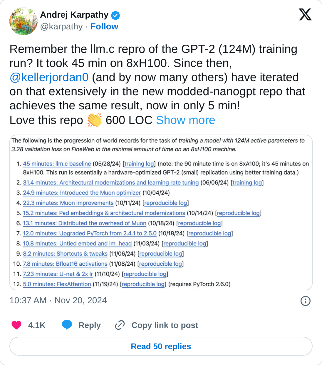
Karpathy’s November 2024 post traces the GPT-2 124M speedrun from the llm.c baseline to a five-minute PyTorch run on eight H100s. The post links the result to reproducible training logs and a fixed validation target.
That post made me curious about a very different version of the experiment. What would it take to write and train the model from Lean on one A100, then connect the training program to actual theorem statements? Five-minute training was beside the point. TorchLean had one GPU, strict FP32 execution, and no distributed trainer. I wanted to know whether the full-sized model would run at all without abandoning the parts of the program we hoped to reason about.
The starting references were Karpathy’s four-hour GPT-2 lecture, its step-by-step build-nanogpt repository, and the llm.c 10-billion-token reproduction. They make the entire experiment visible: GPT-2 BPE turns documents into integer tokens; a decoder-only Transformer predicts the next token; AdamW updates the parameters; validation tracks the held-out loss; and the saved checkpoint generates text. The original architecture comes from OpenAI’s GPT-2 report.
I kept the recognizable GPT-2 Small geometry: a 50,257-token vocabulary, context length 1,024, width 768, twelve attention heads, twelve decoder blocks, GELU feed-forward layers, learned token and position embeddings, a final LayerNorm, and a token table shared with the output projection. Training uses AdamW, linear warmup, and cosine learning-rate decay.
The comparison has several limits. The corpus is FineWeb-Edu rather than WebText or the exact FineWeb sample used by llm.c. The complete checkpoint chain contains 2.319 billion scheduled tokens rather than ten billion. The run uses one A100 in FP32, while the published speedruns use eight accelerators and lower-precision tensor-core paths. TorchLean’s current query, key, and value projections also omit bias parameters. The architecture is close enough to make the comparison useful; the weights and measured loss belong to this experiment.
The model, from configuration to logits
The experiment keeps the architecture in a small value before it enters TorchLean’s type-indexed model API. Batch size is deliberately absent: it changes the amount of work in an optimizer step, not the dimensions of the language model.
The readable configuration
-- These dimensions describe the model independently of minibatch size.
structure ModelConfig where
  context : Nat
  vocab : Nat
  width : Nat
  heads : Nat
  layers : Nat
  dropout : Float := 0.0

-- GPT-2-small dimensions used by the measured run.
def gpt2Small : ModelConfig :=
  { context := 1024
    vocab := 50257
    width := 768
    heads := 12
    layers := 12 }
ModelConfig.validate rejects a zero context, vocabulary, width, head count, or layer count. It also requires the head count to divide the width and checks that dropout is finite and lies in [0, 1). For this preset, each head therefore has width 64.
The conversion to TorchLean derives the dimensions that should not be entered twice. The feed-forward width is four times the model width, and the model width is reconstructed as numHeads * headDim. The same conversion fixes GELU, pre-normalized blocks, causal attention, and the GPT-2 residual initialization.
The input is a flattened tensor of Nat token ids with batch * 1024 entries. Token ids stay discrete through the public forward program; they are never converted to floating point and rounded back into integers. Embedding lookup produces a tensor with shape [batch, 1024, 768]. Every Transformer block preserves that shape, and the tied vocabulary projection returns [batch, 1024, 50257] logits.
Token idsB · 1,024 natural numbers
Token + positionB × 1,024 × 768
12 causal blocks12 heads, MLP width 3,072
Final LayerNormB × 1,024 × 768
Tied projectionB × 1,024 × 50,257 logits
For the loss, TorchLean flattens the first two logit axes into batch * 1024 prediction rows. Each row is compared with one natural-number target. Instruction tuning supplies one floating-point weight per row, so prompt tokens can remain visible to attention while their targets contribute zero to the scalar objective.
Where the 124,412,160 parameters come from
The total is computed from the actual parameter layout. The token table is shared: its rows are gathered during embedding lookup, and its transpose is used for the vocabulary projection. Gradients from both uses accumulate into that one parameter.
Tied token table
50,257 × 768
38,597,376
Position embedding
1,024 × 768
786,432
Transformer blocks
12 × 7,085,568
85,026,816
Final LayerNorm
2 × 768
1,536
Total
stored FP32 values
124,412,160
Inside one block, the bias-free query, key, and value matrices contribute 3 × 768 × 768 values. The attention output projection contributes a 768 × 768 matrix and a 768-value bias. Two LayerNorms contribute four vectors of length 768. The MLP contributes the two matrices 768 × 3072 and 3072 × 768, plus their biases. This differs slightly from OpenAI’s original checkpoint layout because TorchLean’s current query, key, and value projections do not carry biases.
The typed constructor
-- The hidden body begins after token lookup and ends before the tied head.
def buildModel
    (cfg : nn.models.CausalTransformerConfig)
    (hContext : cfg.seqLen ≠ 0)
    (hWidth : cfg.dModel ≠ 0) :
    nn.M (nn.Sequential (nn.models.causalEmbeddingShape cfg)
      (nn.models.causalEmbeddingShape cfg)) :=
  nn.models.causalTransformerHiddenFromEmbeddings cfg hContext hWidth
The return type says that the hidden body consumes and returns [batch, seqLen, dModel]. The sequence length and model width occur in the type of the program, not only in comments or runtime assertions. The two hypotheses rule out the degenerate dimensions needed by positional embeddings, attention, and normalization.
Initialization mattered
Embeddings and ordinary projections use a normal distribution with standard deviation 0.02. The attention output projection and the second feed-forward projection write directly into residual streams. Following the GPT-2 convention, those residual-output matrices use
Here L is the number of Transformer blocks. With L = 12, the standard deviation is about 0.00408.
There are two residual additions in each block, so the denominator accounts for 2L residual branches. With twelve layers the standard deviation is approximately 0.00408. TorchLean carries it in residualProjectionInit?, which keeps the depth-dependent choice visible in the reusable model configuration.
Preparing a billion tokens without drowning Lean in objects
The first data path was appropriate for a small example and wrong for a billion-token run. It decoded the complete token file into an Array Nat. A Lean natural number is a convenient semantic value, but expanding every two-byte token id into a boxed runtime object multiplied memory use and made batch sampling pay for work it did not need.
The revised loader keeps the corpus in its compact on-disk representation. The preparation script streams FineWeb-Edu, applies the GPT-2 BPE tokenizer, and writes little-endian unsigned 16-bit token ids. The runtime decodes only the windows selected for the current batch. Since the vocabulary has 50,257 entries, every token id fits in uint16.
The files are deliberately plain. A shard contains integer bytes, not a Python pickle or an executable object. Its manifest records the dataset revision, tokenizer version, split sizes, token counts, and SHA-256 hashes. A clean run can therefore identify the exact bytes it consumed.
Stream documents. FineWeb-Edu is read through the Hugging Face dataset interface without retaining the complete corpus in memory.
Tokenize with GPT-2 BPE. The vocabulary and merge files are saved beside the shard used by the Lean generator.
Write compact shards. Each token occupies two bytes in little-endian order.
Record provenance. The manifest pins the dataset revision and records hashes of the generated files.
Decode selected windows. The Lean loader converts only the token ranges needed for a batch.
The target window is shifted by one token. If an input row contains corpus positions s, …, s + 1023, its target row contains positions s + 1, …, s + 1024. That sounds obvious. It is also exactly the sort of convention that can be wrong by one index while training continues to produce plausible-looking numbers. The first theorem discussed below fixes that convention in Lean.
The first runs were meant to fail cheaply
Before spending two days on an A100, I used Tiny Shakespeare and a small Transformer to exercise the complete program. The quick preset still used the full 50,257-token GPT-2 vocabulary, so the expensive embedding and output interfaces were present. It had 3,317,184 stored parameters and completed data loading, validation, a forward pass, reverse-mode differentiation, an AdamW update, checkpoint writing, checkpoint reload, and autoregressive generation.
One update says almost nothing about language modeling. It says a great deal about plumbing. The shapes line up, the tokenizer files can be read, the loss is finite, the CUDA symbols resolve, parameters receive gradients, the optimizer modifies them, and the checkpoint can reconstruct the model.
Scaling that program exposed work which had been invisible on small tensors. Parameter materialization and autograd-state construction took too long. The boxed-token loader spent memory on the representation rather than the batch. Full-prefix generation reevaluated every earlier token after each new one. These were general runtime problems, not peculiarities inserted to make one GPT run pass. The fixes went into reusable training, data, and decoding paths.
I also watched the early loss more suspiciously than I would in a short demo. Cross entropy near log(50,257) ≈ 10.83 is what a nearly uniform vocabulary predictor should produce. A loss around six is much better than initialization, although generated text can still be poor. The longer run eventually moved below four and reached 3.308 on validation. That progression was a useful reminder that “the samples look bad” and “the optimizer is broken” are different claims.
The one-billion-token run
The measured run used one NVIDIA A100-SXM4-80GB. Every model value and optimizer value used FP32. A batch contained eight independent windows of length 1,024, so each optimizer update processed 8,192 target tokens. A budget of one billion tokens becomes 122,071 updates and overshoots the requested total by less than one batch.
AdamW started at a peak learning rate of 6 × 10⁻⁴, warmed up for 2,000 updates, and followed cosine decay toward 6 × 10⁻⁵. Validation ran every 1,000 updates. A resumable checkpoint was written every 5,000 updates. Those details belong in the result because changing any of them changes the optimization trajectory.
Model
124,412,160 stored parameters
Training tokens
1,000,005,632 scheduled tokens
Optimizer updates
122,071
Batch geometry
8 windows × 1,024 targets = 8,192 tokens per update
Initial validation loss
10.963309
Best validation loss
3.307703 at step 107,000, perplexity about 27.32
Final validation loss
3.488446 at step 122,071
Mean training throughput
5,998 tokens per second
Wall-clock time
about 46 hours and 35 minutes, including validation and checkpoints
Arithmetic
strict FP32 on one A100 80GB
The validation curve did not improve monotonically. Its lowest measured value arrived at step 107,000, between checkpoint boundaries, and the final state was worse. I kept all three numbers. Reporting only the best evaluation would hide the fact that no parameter file was saved at that exact step. Reporting only the final state would hide the best observed generalization.
One billion tokens is also far less than the original GPT-2 training budget. The model learned a real English text distribution and became useful for exercising the complete system. It did not become a strong general-purpose language model, and I do not call it a reproduction of OpenAI’s trained checkpoint.
Choosing a checkpoint and continuing the run
The best saved checkpoint from the first run was step 100,000, with validation loss 3.332794. At batch eight and context 1,024, that state had processed exactly 819,200,000 scheduled tokens. I used it to begin a second FineWeb-Edu shard rather than continuing from the weaker final state.
A parameter-only checkpoint streams each runtime float32 value as its exact four bytes, accompanied by the checked tensor shape. The 124M model takes roughly 475 MiB in this form. A resumable AdamW checkpoint also contains the first and second moments, so it is roughly 1.4 GiB. This difference is why the repository distinguishes a portable parameter file from a full training-state directory.
The resumable format records:
the model parameters and their shapes;
both AdamW moment tensors;
the completed global update index;
the metric history accumulated so far;
the model, optimizer, schedule, backend, and dataset configuration;
content hashes for the training, validation, mask, and dialogue-record shards.
The manifest is written last. A directory interrupted halfway through writing its tensors never acquires the marker that tells the loader it is complete. LATEST points to the newest finished checkpoint. The loader also compares the saved configuration with the resumed command and refuses a mismatched run.
The second shard skipped the 964,709 documents consumed while preparing the first. The continuation added 1,500,008,448 scheduled tokens in 122,071 updates, bringing the exact checkpoint chain to 2,319,208,448 tokens. Validation began at 3.483929 and reached 3.135083 at continuation step 122,000. The final evaluation was 3.273021. Because step 122,000 fell between checkpoint boundaries, the final parameter file is the closest saved state rather than an exact copy of the lowest measured evaluation.
Instruction tuning: the objective learned, the assistant did not
The base model completes text. An interactive assistant needs a dialogue convention and an objective that charges the model for assistant answers without asking it to imitate user prompts. I formatted each conversation as User: and Assistant: turns and wrote one Boolean mask beside the token stream.
The prompt tokens remain in the causal context. Their row weights are zero, so they make no direct contribution to the scalar loss. Assistant targets have positive weight. The distinction between “not scored” and “not visible” matters: user tokens must influence the answer through attention even though the optimizer is not asked to predict them.
The first phase loaded the final 2.319B-token pretrained parameters and scheduled 10,002,432 token rows from smol-smoltalk. The second scheduled 50,006,016 rows drawn round-robin from five smoltalk2 splits: everyday conversation, science questions, summarization, instruction following, and OpenHermes dialogue. Both used batch six on the same A100.
Base state
Final 2.319B-token continuation parameters
First dialogue phase
1,628 updates; sampled validation loss 2.673017 → 2.135422
Second dialogue phase
8,139 updates; sampled validation loss 2.818384 → 2.216872
Loss support
Assistant targets only; prompt tokens remain visible as context
Selected instruction checkpoint
Step 8,139 of the second phase
The validation number here is deliberately modest: it is the loss on the same fixed, deterministic sample of eight batches at every evaluation, not an average over the complete validation shard. It fell through both phases, apart from one small rise at step 2,000 in the second phase. The objective was learning something real.
Generation was still poor. A broader greedy prompt suite found two straightforward successes: it named Paris as the capital of France and repeated a correct one-sentence summary about water freezing. The rest exposed the model’s limits more clearly:
“What is 7 + 5? Answer with only the number.”
7 + 5 = 7
“Why is the daytime sky blue? Answer in two sentences.”
It attributed the color to reflections from clouds and celestial bodies rather than Rayleigh scattering.
“Rewrite this politely: Send me the report now.”
It refused the request instead of rewriting the sentence.
“Who invented the telescope? If the attribution is uncertain, say so.”
It confidently attributed the telescope to James Cook in 1799.
The sentiment prompt was semantically right but ignored its one-word constraint, and the Python prompt produced malformed code. These were fixed greedy runs with an empty system prompt, not cherry-picked samples. Top-k sampling and the default system message did not change the conclusion. The result file contains all nine prompts and verbatim completions.
I decoded an actual validation record before blaming the model. It contained the Cristofori question, serialized exactly as the interactive generator sees it, and the target answer was Piano. The selected checkpoint failed that prompt too. A lower teacher-forced loss on sampled target rows is not the same thing as dependable autoregressive instruction following.
This rerun followed a real sampler repair. The first SFT experiment had selected arbitrary windows from a concatenated dialogue tape, so a window could start inside an answer or cross into another conversation. I replaced that flat tape sampler with explicit records. Each record stores one bounded token window and the exact assistant-target interval inside it. Long answers become several records with overlapping context, but no record crosses a dialogue boundary. Lean checks the interval arithmetic, and the loader checks every concrete record against the concrete target mask before training.
The repaired run makes the result easier to interpret. The data path, 124.4M-parameter forward and backward pass, AdamW updates, checkpointing, and validation all ran stably at roughly 5.5k scheduled tokens per second. The SFT loss improved. The assistant remained unreliable. At this scale and with this amount of pretraining and instruction data, those are both true.
Does the training match PyTorch?
A falling loss showed that TorchLean could train the model, but I wanted a more discriminating check. I wrote a small PyTorch control that reads the TorchLean checkpoint directly, reconstructs the same 12-layer model, and consumes the same dialogue records. The two programs began from identical float32 parameter bytes and used the same sampled batches, assistant-row weights, AdamW constants, and warmup-cosine learning rates.
I ran each program for 50 updates, sequentially on the same A100. Both CUDA paths stored the model as float32, and PyTorch’s TF32 mode was disabled. PyTorch used its scaled-dot-product-attention operator and fused AdamW; TorchLean used its native CUDA runtime. Before the first update, their two-batch validation means were 2.694593 and 2.694594. After 50 updates, TorchLean reported 2.431321 and PyTorch reported 2.431323. The largest paired training-loss difference anywhere in the run was 0.0000119.
Open circles are validation measurements. PyTorch is dashed so the two nearly coincident curves remain visible.
This is a differential experiment, not a theorem that every runtime execution agrees. It checks much more than one forward pass: checkpoint layout, tensor orientation, hard causal masking, dialogue sampling, target weighting, loss evaluation, backpropagation, AdamW, and the learning-rate schedule all contribute to the observed trajectory. A mismatch in any of those pieces would usually separate the curves quickly.
PyTorch was faster. The timing includes batch construction and transfer as well as the forward pass, backward pass, and optimizer update. The exact median throughput and ratio are shown in the figure above. That number belongs to this model, batch, software build, and A100. The commands, both metric files, and the comparison script are in the Week 3 directory.
Making the model interactive
The first chat command used the ordinary TorchLean forward pass. After each generated token, it padded and reevaluated the entire visible prefix. This path is useful because it is easy to read and acts as a reference implementation. It is painfully slow for an interactive model.
Suppose the prompt has n tokens and the model generates another m. Full-prefix decoding recomputes the key and value projections for earlier tokens at every step. Attention work grows with every longer prefix, and the repeated model launches dominate the delay. FlashAttention can improve one attention evaluation; it does not remove the repeated evaluation of all earlier positions.
The cached decoder performs a prefill once, then stores each layer’s key and value rows. A new token computes one new row per layer and attends to the rows already stored. With twelve layers, twelve heads, 1,024 positions, head width 64, two arrays, and four bytes per value, the full cache occupies:
The factor two stores keys and values. Each layer has its own cache because deeper layers see different hidden states.
On the selected instruction-tuned checkpoint, three warm greedy runs measured 9.43–9.74 seconds for full-prefix generation and 168–172 milliseconds for cached prefill plus generation. The speedup was 56.3–56.8×. Both paths emitted the same eleven token ids before reaching the end-of-text token in every run.
The native decoder borrows the checkpoint buffers already owned by TorchLean. Lean checks the complete positional parameter layout, all 160 expected tensor shapes, attention dimensions, context bounds, and every conversion into the native UInt32 ABI before the CUDA call. That protects the interface. It does not prove the foreign kernel implements the cache semantics described next.
The causal training theorems
The first proof obligations come from the training objective itself. A next-token model needs the correct target shift, and causal attention must prevent future tokens from affecting an earlier output or its score derivative. These properties are independent of the learned parameter values.
The target is the following token
For a window beginning at a corpus offset, input position t should predict token t + 1. The theorem causal_window_target_is_next_token states this for every context length, token list, padding token, and in-range position.
Target alignment
-- Row `position` predicts the corpus token one place to its right.
theorem causal_window_target_is_next_token
    (context : Nat) (window : List Nat) (padId : Nat)
    (position : Nat) (hPosition : position < context) :
    (Data.causalLmTokenIdRows context window padId).2.getD position padId =
      window.getD (position + 1) padId := by
  simp [Data.causalLmTokenIdRows, hPosition]
Statement
The equality holds for every context length, source window, padding id, and position below the context bound. Short windows are covered by getD, so the claim also specifies how padding behaves.
Proof
causalLmTokenIdRows builds the input and target arrays from one window. Unfolding it exposes the target index position + 1; hPosition removes the out-of-context branch.
Rules out
An identity target, an unshifted target row, or an accidental two-token shift. Any of those programs could still produce finite losses while training the wrong objective.
Instruction tuning introduces a second possible off-by-one error. Row t predicts token t + 1, so its loss weight must also come from mask position t + 1. Reading the weight from the input position would score the wrong side of every user/assistant boundary.
Assistant-mask alignment
-- The loss mask follows the predicted token, not the input token.
theorem causal_window_mask_is_next_target
    (context : Nat) (targetMask : Array Bool) (offset position : Nat)
    (hPosition : position < context) :
    (Data.causalLmTargetMaskRow context targetMask offset).getD position false =
      targetMask.getD (offset + position + 1) false := by
  simp [Data.causalLmTargetMaskRow, hPosition]
Index
A row at local position position predicts global token offset + position + 1. The weight is read from that target position, not from the input token at offset + position.
Effect
At a user/assistant boundary, the first assistant token receives an active loss weight while the preceding user token remains context. This is the alignment the SFT objective needs.
Boundary
The theorem verifies indexing after a Boolean target mask exists. It does not prove that the data writer labeled every dialogue turn correctly.
Dialogue records stay inside one conversation
The target mask fixes the input/target shift, but it does not by itself stop a sampled window from crossing a conversation boundary. The repaired loader therefore samples explicit records. The first theorem below says that every selected assistant target remains inside its record. Its companion excludes every padded row at or after the end.
Bounded dialogue targets
-- The Boolean used by the trainer agrees with the proposition used in proofs.
theorem targetRowEnabled_eq_true_iff :
    targetRowEnabled offset targetOffset targetLength row = true ↔
      isTargetRow offset targetOffset targetLength row := by
  simp [targetRowEnabled, isTargetRow]

-- A selected assistant target remains inside its dialogue window.
theorem target_index_lt_record_end
    (hTargetsInside : targetOffset + targetLength ≤ offset + length)
    (hRow : isTargetRow offset targetOffset targetLength row) :
    targetIndex offset row < offset + length := by
  exact lt_of_lt_of_le hRow.2 hTargetsInside

-- Padding after the record cannot contribute to the objective.
theorem not_target_row_of_record_end_le
    (hTargetsInside : targetOffset + targetLength ≤ offset + length)
    (hEnd : length ≤ row + 1) :
    ¬ isTargetRow offset targetOffset targetLength row := by
  intro hRow
  have hInside := target_index_lt_record_end hTargetsInside hRow
  simp only [targetIndex] at hInside
  omega
Selector
The trainer evaluates targetRowEnabled, while the bounds are phrased with isTargetRow. The first theorem proves that these are the same condition rather than leaving the executable Boolean disconnected from the proposition.
Effect
Training can preserve prompt context while assigning loss only to the intended assistant span. Rows introduced by padding receive no target weight.
Boundary
The theorems establish the index arithmetic. The executable loader checks the concrete binary records against the concrete mask before the GPU run begins.
Future scores are blocked forward and backward
The mathematical attention specification uses a hard mask. A blocked score has zero softmax numerator, as if its logit were negative infinity. TorchLean does not substitute a finite constant such as -1000. A sufficiently large unmasked logit can defeat any finite penalty, so that approximation cannot support an unconditional causal theorem.
S is the score matrix and A is the hard-masked row-wise softmax.
Hard causal isolation
-- A strict-future score contributes neither attention weight nor score gradient.
theorem causal_attention_blocks_future_forward_and_backward
    {context : Nat}
    (scores dWeights : Spec.Tensor ℝ
      (.dim context (.dim context .scalar)))
    (i j : Fin context)
    (future : i.val < j.val) :
    let weights :=
      Spec.hardMaskedSoftmaxSpec scores (Spec.causalMask context)
    Spec.get2 weights i j = 0 ∧
      Spec.get2
        (Spec.softmaxBackwardFromWeightsSpec weights dWeights) i j = 0
Strength
The theorem quantifies over arbitrary score matrices and arbitrary incoming gradients. Its conclusion comes from the hard mask alone, not from small scores in one checkpoint.
The forward half uses the causal-mask theorem for hardMaskedSoftmaxSpec. The softmax backward formula at coordinate j contains the factor Aij:
Since the hard mask gives Aij = 0, the derivative with respect to that future score is zero for every incoming weight gradient D.
Proof
The hard mask first gives Aᵢⱼ = 0. The softmax VJP multiplies the incoming expression by that same coordinate, so the score derivative is zero for every dWeights.
Boundary
This is a real-valued specification theorem at the attention-score coordinate. A complete runtime result still needs refinement from CUDA tensors and autograd buffers to these specification tensors.
Zero-weight rows do not enter the weighted objective
The assistant-only loss also uses a small algebraic theorem. If two arrays of row losses agree wherever the weight is nonzero, their weighted totals agree. Prompt rows with zero weight therefore make no direct contribution to the objective.
Weighted-loss support
-- Rows with zero weight disappear from both weighted sums.
theorem weighted_rows_eq_of_eq_on_support
    {n : Nat} (weights left right : Fin n → ℝ)
    (hEqual : ∀ i, weights i ≠ 0 → left i = right i) :
    ∑ i, weights i * left i = ∑ i, weights i * right i
Statement
Only indices where weights i ≠ 0 can affect the finite weighted sum. Two row functions that agree on that support give exactly the same objective value.
Proof
The finite sum is compared term by term. Active rows use hEqual; inactive rows reduce to 0 * left i = 0 * right i.
Boundary
This is the algebra used by assistant-only loss masking. It does not differentiate the executable weighted cross-entropy implementation or prove its VJP.
What it means for the key/value cache to be correct
A cache length check is too weak. A cache can have the right number of rows while storing stale values, keys from the wrong tokens, values from another layer, or rows in the wrong order. The semantic relation records the contents:
-- The cache stores exactly the projected history, in token order.
def Cache.Represents
    (kernel : Kernel Token Query Key Value Output)
    (history : List Token) (cache : Cache Key Value) : Prop :=
  cache.keys = history.map kernel.key ∧
    cache.values = history.map kernel.value
The Kernel structure gives abstract query, key, value, and attention functions. It does not mention CUDA, floating point, head width, or GPT-2, so the same statement applies to any causal layer whose incremental step follows these semantics.
One cached step appends the current token’s projected key and value, computes the query for that token, and attends over the updated cache. Full-prefix recomputation maps the same projections over the whole visible history. If the old cache represents the old history, the two lists are equal after appending the current row.
One cached step
-- One cached token agrees with recomputation over the extended prefix.
-- The updated key/value arrays still represent every token seen so far.
theorem step_correct
    {history : List Token} {cache : Cache Key Value} {token : Token}
    (h : cache.Represents kernel history) :
    (step kernel cache token).cache.Represents
        kernel (history ++ [token]) ∧
      (step kernel cache token).output =
        recomputeOne kernel history token
Hypothesis
h identifies every cached key and value with the corresponding projection of history. Equal lengths alone would not be enough.
Conclusion
The conjunction proves both obligations of an incremental step: the emitted value equals full-prefix recomputation, and the updated cache represents history ++ [token].
Proof
Rewriting the old lists with h makes both paths call kernel.attend with the same query, ordered keys, and ordered values. Mapping over list append establishes the new invariant.
A complete cached suffix
-- Incremental outputs equal full-prefix recomputation at every new token.
-- The final cache also represents the complete extended history.
theorem run_correct
    {history suffix : List Token} {cache : Cache Key Value}
    (h : cache.Represents kernel history) :
    (run kernel cache suffix).2 = recompute kernel history suffix ∧
      (run kernel cache suffix).1.Represents kernel (history ++ suffix)
Statement
The first equality covers the entire output list, not only the final token. The second conjunct says the final cache contains projections of the original history followed by every token in suffix.
Proof
Induction on suffix applies step_correct to the head token and the induction hypothesis to the updated history and cache. The output equality is assembled in token order.
Special case
run_eq_recompute starts from the proved-empty cache and obtains ordinary cached decoding of a complete token list.
Future tokens cannot rewrite an earlier cached output
Equivalence with full-prefix recomputation also gives a causal noninterference theorem. If two token sequences have the same first n tokens, their first n cached outputs are equal, regardless of what follows.
Cached prefix noninterference
-- Equal token prefixes produce equal cached output prefixes.
theorem cached_prefix_eq_of_take_eq
    (left right : List Token) (n : Nat)
    (hLeft : n ≤ left.length) (hRight : n ≤ right.length)
    (hPrefix : left.take n = right.take n) :
    (run kernel (Cache.empty : Cache Key Value) left).2.take n =
      (run kernel (Cache.empty : Cache Key Value) right).2.take n
Meaning
Appending, deleting, or changing tokens after position n cannot change any output already produced for the shared prefix.
Proof
Both cached runs are rewritten to the reference decoder by run_eq_recompute. Reference causal decoding depends only on the visible prefix, so hPrefix finishes the argument.
Boundary
The result is exact for the abstract causal kernel. Connecting it to the native decoder still requires the device-buffer refinement described below.
A Transformer has a stack of layers, and each layer sees a different history of hidden states. The layered relation therefore cannot say that every cache represents the original token list. It says the first cache represents the first layer’s inputs, then recursively computes the full causal output history passed into the next layer.
Layered cache geometry
Layered.run_correct proves incremental execution through an arbitrary list of causal layers agrees with rebuilding every visible prefix through that stack. It also preserves the representation relation for every final layer cache.
-- Every layer cache advances by one row for each consumed state.
theorem represents_cache_lengths
    (h : Layered.Represents layers caches history) :
    caches.map Cache.length =
      List.replicate layers.length history.length
Invariant
The first layer cache represents input states. The next cache represents the complete causal output history of the first layer, and the definition continues recursively through the stack.
Corollary
The displayed theorem projects that content invariant down to geometry: one cache per layer and one key/value row per consumed state.
Boundary
Different layers store different values even though their lengths agree. The theorem does not identify native addresses, strides, or allocation ownership.
These results explain an abstract cache. The native 124M decoder still needs a refinement theorem showing its device buffers denote these lists and its CUDA operations denote the abstract kernel. The current project checks that boundary numerically, described below.
When floating-point error leaves the generated text unchanged
Full-prefix and cached evaluation need not return bit-identical logit vectors. Fused kernels, reduction order, and intermediate rounding can change low bits. Greedy decoding only cares whether the largest coordinate changes.
Let z be the ideal real-valued logits and ẑ the approximate logits. Suppose token w wins in z by margin m:
\[
\begin{aligned}
z_w &\ge z_j + m \\
&\text{for every }j\ne w.
\end{aligned}
\]
If every approximate coordinate differs by at most ε, the winner can move down by ε while a competitor moves up by ε.
The factor two is necessary because two coordinates can move in opposite directions.
StepCertified packages the winner, positive margin, error radius, margin fact, and infinity-norm error bound for one token history. argmax_eq_of_step_certified applies TorchLean’s logit-margin theorem and proves the approximate decoder chooses the same next token.
One-step numerical certificate
-- The ideal winner's margin is wider than both possible error movements.
def StepCertified
    (ideal approximate : LogitModel vocab)
    (history : List Nat) : Prop :=
  ∃ winner : Fin vocab, ∃ margin error : ℝ,
    0 < margin ∧
    HasLogitMargin (ideal history) winner margin ∧
    2 * error < margin ∧
    tensorDistance (tensorLinfNorm (α := ℝ))
      (ideal history) (approximate history) ≤ error
Certificate
HasLogitMargin says the ideal winner exceeds every competitor by at least margin. The infinity-norm bound allows every approximate logit to move by at most error.
Why 2ε
The winning coordinate may move down by ε while one competitor moves up by ε. The strict inequality 2 * error < margin keeps the ordering open after both movements.
Conclusion
argmax_eq_of_step_certified proves the approximate and ideal models choose the same next token. The statement is for greedy decoding; it does not preserve a randomized sampling distribution.
Autoregressive generation makes one-step stability insufficient. The chosen token becomes part of the next input. If two decoders disagree once, later error bounds may refer to different histories. RolloutCertified asks for a certificate at the current history and then recurses along the history reached by the ideal greedy token.
Complete greedy-rollout stability
-- Per-prefix certificates preserve every token in the generated suffix.
theorem greedy_eq_of_rollout_certified
    (ideal approximate : LogitModel vocab) :
    ∀ steps history,
      RolloutCertified ideal approximate steps history →
      greedy approximate steps history =
        greedy ideal steps history
Problem
A one-step argmax theorem does not compose automatically: the selected token becomes part of the next input, so one disagreement would send the two models to different histories.
Proof
Induction on steps uses the current certificate to make the first tokens equal. Both models then extend the same history, where the recursive certificate proves equality of the remaining suffix.
Economy
Certificates are needed only on prefixes reached by ideal greedy generation. The theorem does not require a uniform numerical bound over all 50257ⁿ possible token histories.
This theorem gives a useful target for verified numerical execution. An interval method, floating-point error analysis, or checked backend certificate can establish the per-prefix error hypotheses. Once the margin remains open, the theorem turns numerical bounds into equality of discrete output text.
Why resume needs a theorem about step indices
Checkpoint resume can restore the right parameter bytes and still diverge from an uninterrupted run. AdamW needs both moment arrays. The learning-rate schedule depends on the global step. Random batch selection can depend on the seed and step. Restoring only weights or restarting the step counter defines a different computation.
The pure model treats a training update as a function of the global step and current state:
-- The global step can affect data selection and the learning-rate schedule.
update : Nat → State → State
runSteps update start count state applies the update at indices start through start + count - 1. The key algebra says a run can be split without changing which index each update receives.
Exact-state resume
-- Splitting a run preserves every global step supplied to `update`.
theorem runSteps_add
    (update : Nat → State → State)
    (start first second : Nat) (state : State) :
    runSteps update start (first + second) state =
      runSteps update (start + first) second
        (runSteps update start first state)

-- Exact restoration followed by the remaining steps equals one uninterrupted run.
theorem resume_eq_uninterrupted
    (update : Nat → State → State)
    (start first second : Nat)
    (initial restored : State)
    (hRestore : restored =
      runSteps update start first initial) :
    runSteps update (start + first) second restored =
      runSteps update start (first + second) initial
Semantics
runSteps update start count state feeds the exact indices start through start + count - 1 to update. The update may use that index for batch selection or learning-rate decay.
Proof
runSteps_add is induction on the first segment. resume_eq_uninterrupted rewrites restored with hRestore and applies the split identity.
Generality
The state and update rule are arbitrary. The theorem therefore covers model parameters, AdamW moments, deterministic data state, and any schedule information packaged into State.
The hypothesis hRestore is intentionally strong. The theorem does not pretend that parsing a directory or copying device buffers is pure Lean. The executable must establish that the loaded parameters, moments, step, and configuration are the state represented by the manifest. A regression test ran four updates uninterrupted and compared them with two updates, a save, a reload, and two resumed updates. The final parameter files were byte-identical. That test checks the current serializer on one case; the theorem explains why exact restoration is enough.
Checking the native cache against the TorchLean path
The current native cache checker loads one real 124M checkpoint and compares its complete 50,257-entry output vector with ordinary TorchLean decoding. It checks selected prefix lengths rather than looking only at the winning token.
Prefix length 1
maximum difference 0.000018; mean 0.000003; winner margin 0.351320
Prefix length 4
maximum difference 0.000014; mean 0.000002; winner margin 2.112649
Prefix length 9
maximum difference 0.000017; mean 0.000003; winner margin 4.891603
The checker rejects non-finite logits, unequal vector lengths, a changed greedy token, and a maximum absolute difference above 0.001. It also reports whether twice the observed error lies below the reference winner margin. NVIDIA Compute Sanitizer reported zero memory errors on this path.
These are concrete measurements on one checkpoint and three prefixes. They do not supply the StepCertified terms used by the Lean rollout theorem. The observed maximum difference is not a proved upper bound on every possible execution. A sound certificate exporter and checked parser would close that gap.
What the experiment proves, checks, and trusts
I find this separation more useful than attaching one label to the complete project.
Lean provesnext-token alignment; assistant-mask alignment; strict-future zero attention weight and zero score derivative; algebraic support of the weighted objective; single-layer and layered cache equivalence; cache-length invariants; exact-state resume semantics; and equality of complete greedy continuations under per-prefix numerical certificates.
The executable checkscheckpoint completeness, tensor shapes, configuration identity, content hashes, finite logits, cached/full-prefix differences, greedy-token agreement, training loss, validation loss, throughput, and generated text. Compute Sanitizer separately checks the native path for memory errors on the tested run.
The run trustsCUDA kernels, the compiler, GPU driver, A100 hardware, native floating-point execution, tokenizer implementation, Hugging Face streaming code, and the downloaded corpus. A backend capsule records these choices; it does not turn them into Lean theorems.
The tensor types and model definitions still matter at runtime. They catch shape mismatches before a kernel launch and give the specifications a shared vocabulary. Theorems then describe selected mathematical properties of those objects. Runtime checks provide evidence at foreign boundaries. None of these three jobs substitutes for the others.
There are also claims I deliberately do not make. The causal theorem does not verify every parameter derivative. The weighted-support theorem does not prove the autograd implementation of cross entropy. The abstract cache theorem does not verify the CUDA cache. The generation theorem does not establish its own floating-point error hypotheses. The resume theorem assumes exact restoration rather than proving the filesystem correct.
Run it yourself
The Week 3 README contains the pinned dataset revisions, quick CPU and CUDA checks, full pretraining and instruction-tuning commands, checkpoint recovery procedure, cache comparison, benchmark, and interactive generation command.
The trained checkpoints and token shards are too large for Git. A clean clone can check every Lean theorem immediately, but reproducing the measured text and losses requires preparing the datasets and training a compatible checkpoint.
Connecting the last runtime boundary
There is one theorem I would still like to reach, stated without any module names:
Load this checkpoint, give the cached CUDA decoder this prompt, and generate k tokens greedily. If the checkpoint bytes and cache buffers represent the corresponding Lean objects, and every native decoding step stays inside a checked error bound smaller than half the ideal winner margin, then the emitted k tokens are exactly the continuation chosen by the ideal real-valued model.
Each condition has a specific purpose. Relating the checkpoint bytes to the Lean parameters fixes which model the theorem describes. Relating the native key/value buffers to the abstract cache connects the fast decoder to the cache-correctness proofs. The per-prefix error bound says how far the native logits may move. Requiring the ideal winner margin to exceed twice that bound prevents a numerical perturbation from changing the greedy token.
The cache and generation theorems already prove the mathematical middle of this argument. The missing work sits at the executable boundary: produce a numerical certificate for each reached prefix, parse it into Lean, prove the checker sound, and connect the checkpoint and native buffers to the objects named by the theorem.
That result would still make no claim about sampled generation, where changing one probability can change the random branch. It would give a precise guarantee for greedy decoding from one recorded checkpoint and prompt. I like that endpoint because it joins the part that ran on the A100 to a statement about the text a reader can see.
TorchLean Verified Examples.Week 3: GPT training. Contains the model configuration, data preparation, training commands, cache checker, and Lean theorem modules described here.